Mixed Integer Linear Programming
The typical flow of thought undergoing in a human mind is constantly planning the things to be done: within a certain time-frame, before the deadline, increasing profits, minimizing the travel redundancies along-with routine survival chores. Such parallel processing and/or planning are not yet mastered by robots. The field of mathematics which deals with this situation is Mathematical Optimization a.k.a. Linear Programming.
*Keywords:* Operations research, mathematical optimization, linear programming, mathematical modeling
Introduction
In the context of mathematical optimization, the term “programming” refers to the concept of planning. When the equations involved in the optimization problem are linear, we speak of “linear programming”. The technique of linear programming was first invented by the Russian mathematician L. V. Kantorovich and developed later by George B. Dantzig. NEOS Guide [1] provides an optimization taxonomy, reported in Figure, focused mainly on the subfields of deterministic optimization with a single objective function.
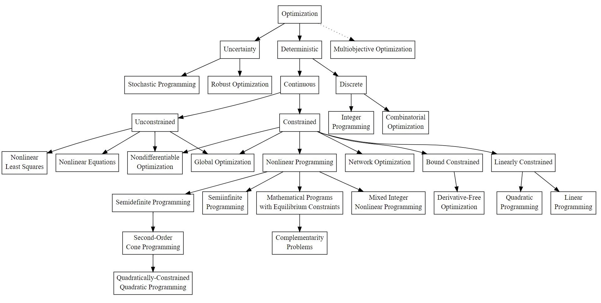
Linear programming deals with optimization problems that are deterministic, continuous and linearly constrained.
A linear programming problem is one in which some function is either maximized or minimized relative to a given set of alternatives. The function to be minimized or maximized is called the objective function and the set of alternatives is called the feasible region determined by a system of linear inequalities (constraints). Mixed integer refers to the combination of integers and continuous decision variables.
Below is an example of a MILP model.
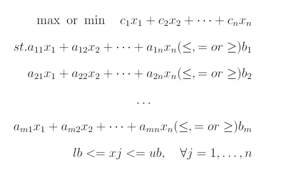
Equation 1 represents the objective function of the formulation, where c_i are the coefficients making the linear objective function and x is the decision variable (output of the solver). This objective is subject to a set of requirements which are enforced as *constraints*. As per these constraints, decisions are made which becomes the value of the *decision variable*. Equations 2-4 combines the equality and inequality constraints of the model. Finally, Equation 5 encode the upper and lower value bound of each decision variable.
Discussion
“Since all linear functions are convex, linear programming problems are intrinsically easier to solve than general nonlinear (NLP) problems, which may be non-convex. In a non-convex NLP, there may be more than one feasible region and the optimal solution might be found at any point within any such region. In contrast, an LP has at most one feasible region with 'flat faces' (i.e. no curves) on its outer surface, and the optimal solution will always be found at a 'corner point' on the surface where the constraints intersect. This means that an LP Solver needs to consider many fewer points than an NLP Solver, and it is always possible to determine (subject to the limitations of finite precision computer arithmetic) that an LP problem (i) has no feasible solution, (ii) has an unbounded objective, or (iii) has a globally optimal solution (either a single point or multiple equivalent points along a line).”
The flexibility of MILP is what makes them the widely preferred method [2] in process scheduling problems. However, consider a model has $n$ binary variables, there would be $2^n$ possible configurations to search from. There are several techniques to speed up the generation of an optimal solution. One of them is the *Branch and Bound* technique. Initially, the integrality restrictions are removed and the problem is solved as a Linear Programming (LP) problem. This is known as *LP relaxation* of the original MILP. Usually, a perfect fit for the original problem is not found by simply relaxing the integer constraints. The next step is to select some variable (restricted as an integer), whose optimal value in the LP relaxation is fractional. This becomes the branching variable and we get two different branches, this process is continued till a solution is found which fits the integer bounds, which can be considered the best solution found so far known as *incumbent*. The generated search tree is explored for other such solutions having better values of the objective function. If they exist we have an *optimality gap*, otherwise, we have found our optimal solution. The practitioner can also improve the computation runtime by providing integer bounds in the constraint set of the model despite defining them while the decision variable declaration. This helps in tightening the formulation by removing undesirable fractional solutions, termed as *cutting planes*. Some solvers use pre-existing knowledge of the defined problem and tighten the model to get solutions faster. Additionally, *heuristic* algorithms can be applied to sacrifice optimality and find a solution to the problem faster. This technique provides an initial feasible solution or incumbent to kick-start the search of the optimal solution.
Solvers
Several commercial and open source optimization solvers are available in the user can simply focus on formulating the model rather than dealing with details of the actual solution algorithm. Notable software includes IBM ILOG CPLEX Optimization Studio and Gurobi Optimizer. These have optimization IDE as well as support to a model in other languages like C++, Python, MATLAB, R, etc.
- MATLAB
- IBM CPLEX
- Gurobi
- AMPL
- Artelys Knitro for Knitro
- COIN-OR
- FICO for the Xpress Optimization Suite
- GAMS
- Lindo Systems, Inc. for LINDOGlobal
- Mosek
- OpenSolver
Useful Resources
References
[1] “Morgridge Institute for Research and Wisconsin Institute for Discovery, NEOS Server, ”https://neos-guide.org/.
[2] C. A. Floudas and X. Lin, “Mixed integer linear programming in process scheduling: Modeling, algorithms, and applications,” Annals of Operations Research, vol. 139, no. 1, pp. 131–162, 2005.